
Calculus is a branch of Mathematics that deals with the study of ‘Rate of Change’ and their application in solving equations. It has majorly two branches, First one is Differential Calculus that is concerning rates of change and slopes of curves, and the second one is Integral Calculus concerning accumulation of quantities and the areas under and between curves.
Both branches are interconnected through the fundamental theorem of calculus and rely on the fundamental concepts of the convergence of infinite sequences and series towards a precise limit.
Differential Calculus Formulas
Differential calculus is one the branch of mathematics that focuses on the study of properties, definition, and applications of a function’s derivative. The derivative is found through the process of differentiation. To assist with finding the derivative of a function, there are various calculus differentiation formulas. According to definition of differential calculus, the derivative of a function can be determined as follows:
f'(x) = limh→0f(x+h)−f(x)h
Differential Calculus formulas are particularly useful for finding the derivative of a function, and common examples include the power rule, product rule, quotient rule, and chain rules. The important differential calculus formulas for various functions are below:
Elementary Functions
- d/dx ex = ex
- d/dx ax = ax. ln .a , where a > 0, a ≠ 1
- d/dx ln x = 1/x, x > 0
- d/dx √x = 1/(2 √x)
Trigonometric Functions
- d/dx sin x = cos x
- d/dx cos x = -sin x
- d/dx tan x = sec2 x , x ≠ (2n + 1) π / 2 , n ∈ I
- d/dx cot x = – cosec2 x, x ≠ nπ, n ∈ I
- d/dx sec x = sec x tan x, x ≠ (2n + 1) π / 2 , n ∈ I
- d/dx cosec x = – cosec x cot x, x ≠ nπ, n ∈ I
Hyperbolic Functions
- d/dx sinhx = coshx
- d/dx coshx = sin hx
- d/dx tan hx = sec h2x
- d/dx cot hx = -cosec h2x
- d/dx sec hx = -sech hx tan hx
- d/dx cosec hx = -cosec hx cot hx
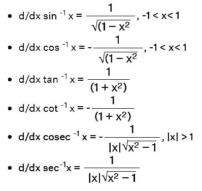
Inverse Trigonometric Functions
Inverse Hyperbolic Functions

Integral Calculus Formulas (Integration Formula)
Integral Calculus is a branch of calculus which deals with finding the integral function, which is the reverse process of finding the derivative. It involves calculating the area under or between curves and is used to solve problems in physics, engineering, economics, and many other fields. Also Integral Calculus formulas include the power rule, substitution rule, integration by parts, trigonometric integrals, and partial fraction decomposition.
These formulas are used to find the antiderivative of a function and evaluate definite integrals by finding the difference between the values of the antiderivative at the endpoints of an interval.
- ∫ xn.dx = xn + 1/(n + 1) + C
- ∫ 1.dx = x + C
- ∫ ex.dx = ex + C
- ∫(1/x).dx = log|x| + C
- ∫ ax.dx = (ax/log a) + C
- ∫ cos x.dx = sin x + C
- ∫ sin x.dx = -cos x + C
- ∫ sec2x.dx = tan x + C
- ∫ cosec2x.dx = -cot x + C
- ∫ sec x.tan x.dx = sec x + C
- ∫ cosec x.cotx.dx = -cosec x + C
Also Check : Trigonometry Table
Definite Integrals Formulas
Definite Integrals is a branch of Integral Calculus that deal with exact value of the area under a curve between two specific points on the x-axis. It’s like measuring the area of a specific region between two points on a graph. The formulas used in Definite Integrals are different from those used in Indefinite Integrals (which find the antiderivative of a function).
The formula for calculating a definite integral involves substituting the upper and lower limits of integration into the antiderivative of the function and subtracting the results. This gives us a precise value for the area under the curve between those two points.
Some common Definite Integrals formulas include the power rule, substitution rule, integration by parts, trigonometric integrals, and partial fraction decomposition. By applying these formulas, we can evaluate the area between two points with great precision.
- ∫ba f'(x).dx = f(b) – f(a)
- ∫ba f(x).dx = ∫ba f(t).dt
- ∫ba f(x).dx = – ∫ab f(x).dx
- ∫ba f(x).dx = ∫ca f(x).dx + ∫bc f(x).dx
- ∫ba f(x).dx = ∫ba f(a + b – x).dx
- ∫a0 f(x).dx = ∫a0 f(a – x).dx
- ∫2a0 f(x).dx = 2∫a0 f(x).dx
- ∫a-a f(x).dx = 2∫a0 f(x).dx, f is an even function
- ∫a-a f(x).dx = 0 , f is an odd function
Vector Calculus Formulas
The Vector Calculus is a branch of mathematics that deals with vector functions and their derivatives, integrals, and other operations of derivatives. Vectors are mathematical objects that have both magnitude and direction, such as velocity or force.
The formulas used in Vector Calculus include the gradient, divergence, curl, and Laplacian operators. These operators are used to calculate different properties of vector fields, such as their direction, rate of change, or potential.
The Vector Calculus formulas are used model physical phenomena, such as fluid flow or electromagnetic fields, and to solve problems in optimization and control theory. Some of the important vector calculus formulas are given below:
From fundamental theorems, we take,
F(x, y, z) = P(x, y, z)i + Q(x, y, z)j + R(x, y, z)k
Fundamental Theorem of Line Integral
If F = ∇f and curve C has endpoints A and B, then
∫c F. dr= f(B) − f(A).
Circulation-Curl Form
Green’s Theorem
∫∫D (∂Q /∂x) – (∂P/ ∂y)dA = ∮C F· dr
Stokes’ Theorem
∫∫D ∇ × F · n dσ = ∮C F· dr, where C is the edge curve of S
Flux – Divergence Form
Green’s Theorem
∫∫D ∇· F dA = ∮C F · n ds
Divergence Theorem
∫∫∫D ∇· F dV = ∯S F · n dσ
Limit Formula
- Ltx→0 (xn – an)(x – a) = na(n – 1)
- Ltx→0 (sin x)/x = 1
- Ltx→0 (tan x)/x = 1
- Ltx→0 (ex – 1)/x = 1
- Ltx→0 (ax – 1)/x = logea
- Ltx→0 (1 + (1/x))x = e
- Ltx→0 (1 + x)1/x = e
- Ltx→0 (1 + (a/x))x = ea
Calculus Formulas and Examples
Derivative Calculus formulas Example:
Find the derivative of f(x) = 3x^2 using the power rule.
Solution: f'(x) = 6x.
Find the derivative of g(x) = (x^2 + 1)(2x – 3) using the product rule.
Solution: g(x) = (2x)(2x-3) + (x^2+1)(2) = 4x^2-6x + 2x^2+2
= 6x^2 – 6x+2.
Integral Calculus formulas Example:
Find the indefinite integral of h(x) = 2x + 3.
Solution: The antiderivative of h(x) is H(x) = x^2 + 3x + C, where C is the constant of integration.
Evaluate the definite integral of i(x) = 3x^2 from x=1 to x=2.
Solution: The antiderivative of i(x) is I(x) = x^3 + C, where C is the constant of integration. Therefore I(2) – I(1) = (2^3 + C) – (1^3 + C) = 7.
Limit Calculus formulas Example:
Find the limit of j(x) = (x^2 – 4)/(x – 2) as x approaches 2.
Solution: We can’t directly evaluate j(2) since it would lead to division by zero. Using algebraic manipulation, we can rewrite j(x) as (x+2), and as x approaches 2, the limit of j(x) is 4.
Find the limit of k(x) = (sin(x))/x as x approaches 0.
Solution: Using the squeeze theorem, we can show that the limit of k(x) as x approaches 0 is 1.


Recent Comments